

This post continues the previous post “Understanding Asset Allocation and the Power of Diversification”
When building an investment portfolio, risk is inevitable. Yet, there’s a powerful tool that allows investors to balance risk and reward strategically: introducing a risk-free asset into the portfolio.
But what exactly is a risk-free asset? Does such a thing really exist? And how can combining risky and risk-free investments help you manage risk while still pursuing attractive returns?
Let’s explore how Modern Portfolio Theory expands when risk-free assets enter the picture—and how this shapes smarter, more resilient portfolios.
What Is a Risk-Free Asset?
First, let’s clarify a common misconception: no investment is truly risk-free. Even the safest financial instruments carry some degree of risk, whether it’s inflation, default, or currency fluctuations.
However, in financial theory, we often refer to instruments such as:
✔ Government bonds from highly rated countries
✔ Treasury bills
✔ Insured bank deposits (up to the guaranteed limit, often €100,000)
These are considered “risk-free” for practical purposes, meaning they carry minimal risk of capital loss and provide stable, predictable returns.
Blending Risky and Risk-Free Assets
Suppose you have a risky portfolio—say, a combination of stocks or mutual funds—and you decide to allocate part of your capital to a risk-free asset. How does this affect your portfolio’s risk and return?
The expected return of this new, blended portfolio is calculated as:
rpf = rc + (rp − rc) × xp
Where:
rpf = Expected return of the new, mixed portfolio
rp = Expected return of the risky portfolio
rc = Return of the risk-free asset
xp = Proportion of capital allocated to the risky portfolio
Breaking It Down:
The formula shows your portfolio’s return is essentially:
The return from your safe asset, plus
The additional “risk premium” earned by investing in risky assets, scaled by how much capital you allocate to them
Risk Premium (rp − rc) is the extra return investors expect for taking on risk beyond what the risk-free asset offers.
Managing Risk: What Happens to Volatility?
Here’s the beauty of adding a risk-free asset:
The risk-free asset has zero volatility (σc² = 0)
The risk-free asset has zero covariance with risky assets (σpc = 0)
This simplifies the overall portfolio risk calculation. Your portfolio’s standard deviation (σpf), which represents its risk, depends only on the portion invested in risky assets:
σpf = σp × xp
Where:
σpf = Expected volatility of the new, mixed portfolio
σp = Expected volatility of the risky portfolio
xp = Percentage of portfolio allocated to the risky assets
Meaning:
The more you allocate to risky assets, the higher the portfolio’s risk
The more you allocate to risk-free assets, the lower the overall risk
Thus, by adjusting your allocation between risky and risk-free assets, you have a direct, controllable way to fine-tune your portfolio’s risk exposure.
Visualizing the Risk-Return Trade-Off
Imagine a graph with:
Risk (volatility) on the x-axis
Expected return on the y-axis
A portfolio entirely invested in risky assets forms a curved line—representing all possible risk-return combinations within that portfolio.
Now, introduce a risk-free asset:
A straight line emerges, starting from the return of the risk-free asset
This line connects to the risky portfolio’s risk-return point
The slope of the line reflects the additional return per unit of risk
This straight line represents all possible combinations of the risky portfolio and the risk-free asset.
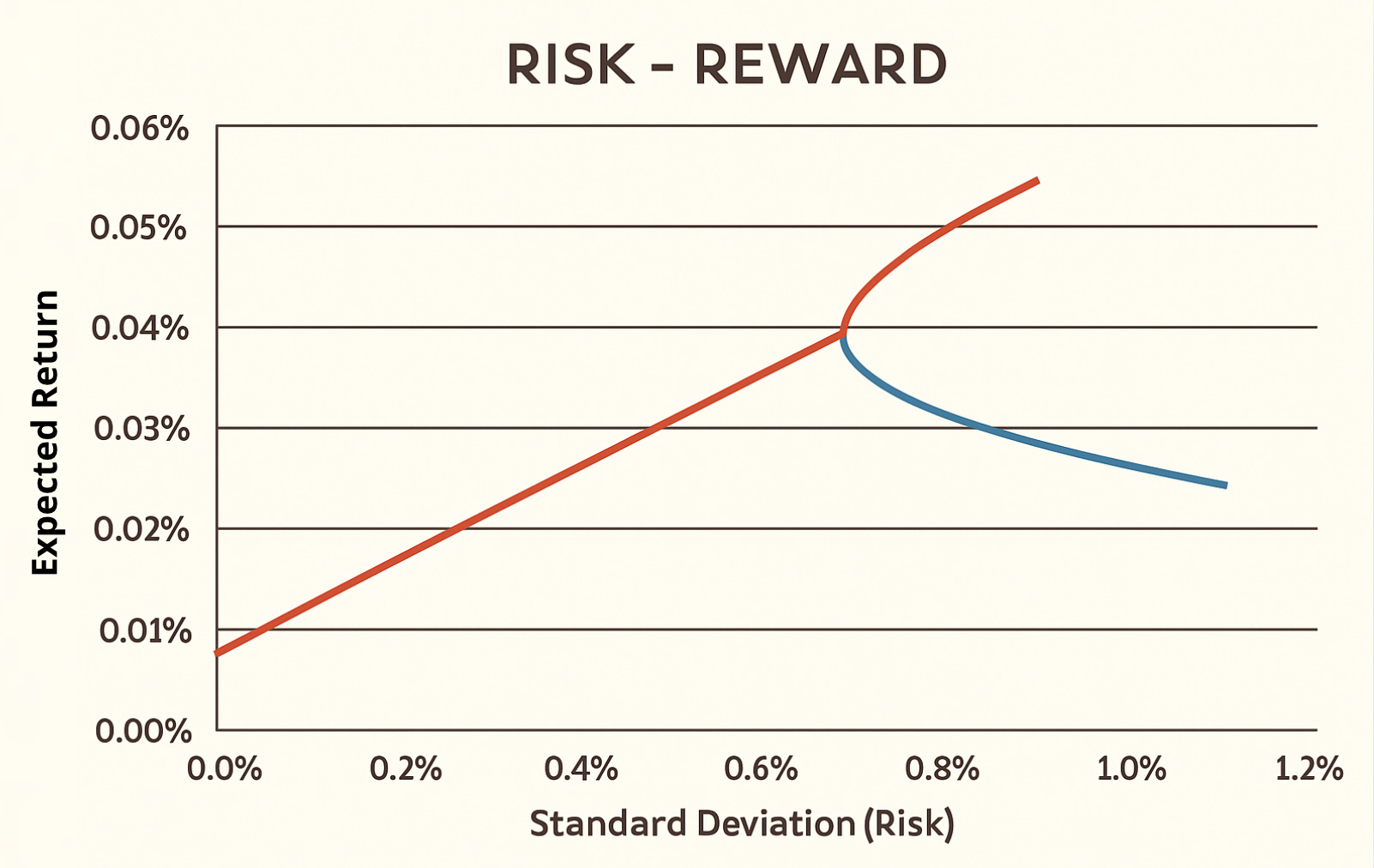
For example:
✔ Investors seeking higher returns can move along the line toward greater risk (higher allocation to risky assets)
✔ More conservative investors stay near the risk-free point, minimizing exposure to volatility
This approach offers an elegant, flexible way to tailor investment strategies based on individual risk tolerance.
Real-World Application
In real-world investing:
Government bonds, such as U.S. Treasuries or German Bunds, often serve as the risk-free component
Balanced portfolios mix equities, funds, or other riskier assets with these safe instruments
The specific allocation depends on market conditions and personal preferences
For example, one portfolio might be made of:
Risky Assets with a chosen percentage:
60% invested in Thailand equities (higher risk)
40% in US equity funds (moderate risk)
Risk-free Assets:
Plus a percentage in government bonds (risk-free component)
By adjusting the proportions, investors can:
✔ Achieve their desired risk-return balance
✔ Enhance the efficiency of their portfolios
✔ Reduce overall volatility without abandoning growth potential
For esample a possible portfolio can be:
48% invested in Thailand equities
32% n US equity funds
20% in government bonds
In this way the proportion inside the risky part is maintained to be 60%-40%.
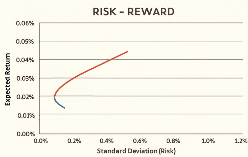
Since in reality there are no risk -free tools with covariance equal to 0 to a basket of risky assets. The graphic designer of the resulting curve is more similar to this:
Beyond Two Assets
Until now we explored only 2 assets portfolio (1 asset and a combination of other assets treated as one). But in practice, portfolios often include more than one risky asset. With multiple funds or stocks:
Correlations between assets matter
Diversification becomes even more powerful
The “efficient frontier” expands, offering more optimal portfolios
The principles remain the same:
Combine risky and risk-free assets
Use diversification to reduce risk
Tailor the portfolio to individual goals
Introducing the Tangency Portfolio and the Sharpe Ratio
The ultimate goal? Find the portfolio that maximizes return per unit of risk.
In financial theory, this is known as the Tangency Portfolio, which:
Lies at the point where the straight line from the risk-free asset is tangent to the efficient frontier
Offers the best possible risk-adjusted return
Becomes the ideal portfolio for combining with risk-free assets
The Sharpe Ratio measures this efficiency:
Sharpe Ratio = (rp − rf) / σp
Where:
rp = Expected return of the portfolio
rf = Risk-free rate
σp = Portfolio volatility
In the following graph the green line has a slope equal to the Sharpe Ratio.
The dot point where the red and the green line intesects is the Tangency Portfolio.
The Tangency Portfolio is the portfolio with the highest return per unit of volatility compared to any other available portfolio. It’s not the best in any case. It’s the best if your risk appetite on reward research is null.
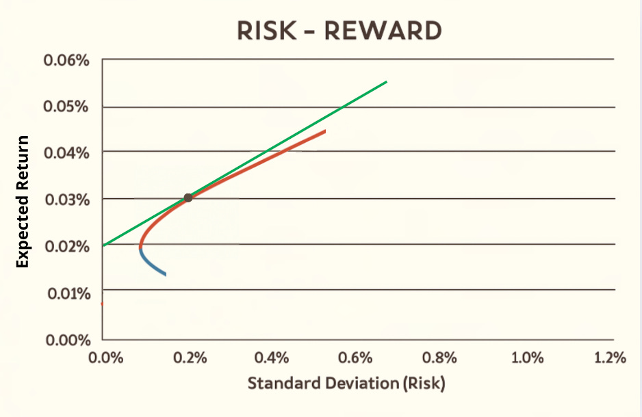
A higher Sharpe Ratio means:
✔ More reward for each unit of risk
✔ A more efficient, desirable portfolio
Final Thoughts: Crafting Smarter Portfolios with Risk-Free Assets
Incorporating risk-free assets isn’t about avoiding risk altogether—it’s about strategic control.
With this approach, investors can:
Design portfolios tailored to their risk appetite
Reduce overall volatility
Optimize returns without unnecessary exposure
Understanding how to mix risky and risk-free investments empowers investors to:
✔ Build resilient, adaptable portfolios
✔ Weather market uncertainty
✔ Pursue long-term financial success with confidence
In investing, safety and risk aren’t opposites—they’re tools to be balanced. Mastering that balance is what sets great investors apart.
Site tip:
If you want to learn more about the math behind the Efficient Frontier Theory —> Geometry of the Efficient Frontier.